Merging related datasets (aka hydrants are awesome)

18 August, 2022, 8 min, 1498 words

Tags: mount-erie-fire gis

Mt. Erie Fire has had a dataset of hydrant locations for many years now, based on data we originally got from Skagit County. We also recently got access to a dataset from one of our mutual aid partners to the north, Anacortes, which includes some of the Public Utility District hydrants they've been taking over of late. The tricky bit: some hydrants are represented in both datasets, with slightly different positions and metadata. This is a summary of how I finally learned how to spatial join in order to construct one dataset of hydrant locations covering both MEFD and Anacortes's service areas.

tl;dr

This is going to be a fairly technical post – effectively the how-to guide I wish I'd had when starting this project. If geospatial analysis isn't your thing, that's cool! But you might want to check out some other content. Or just skip to the fun map at the end.

In short,

1. Hydrants are really important for firefighting (duh).
2. Knowing where hydrants are located is important too.
3. Physical map books are great, but often a digital way of finding nearby hydrants is valuable too. Up until now, while we've had digital hydrant maps for within our district, we relied on mapbooks for mutual aid.
4. A couple weeks ago we got hydrant locations from a frequent mutual aid partner (hooray!), but it also included some hydrants that are in our district. All well and good, but the two datasets didn't quite agree on where these hydrants were.
5. So I did some fun geospatial hackery to combine the datasets into a best understanding of where hydrants are located within our district and outside, in the service area for our mutual aid partner.

Step one: general visualization and recon

With pretty much any dataset, my first move is to find a way to visualize it so I can start to develop intuition. In this case, that meant mapping the two hydrant location datasets and seeing if they matched up at all. The answer: mostly.

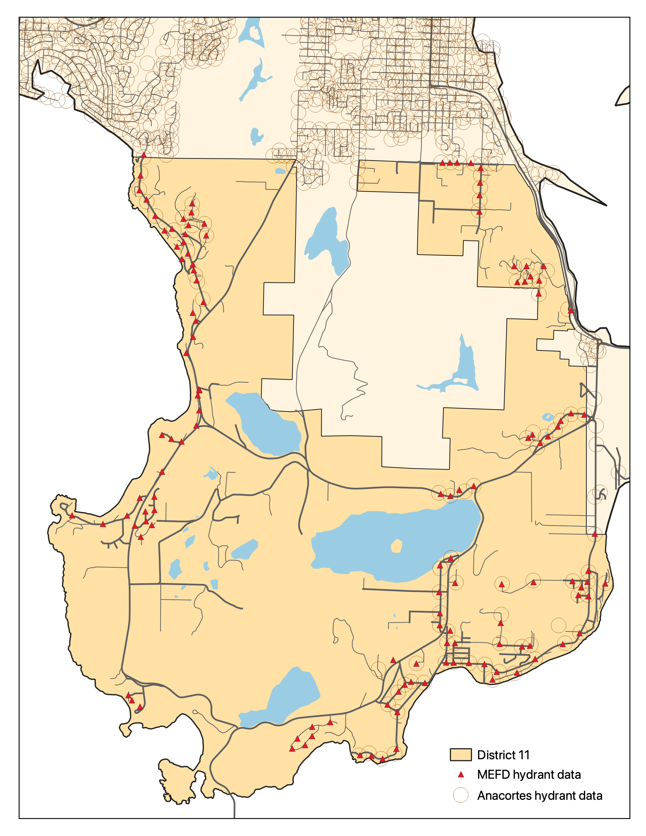
Most places it's clear that either 1) a hydrant is only in one of the datasets or 2) the hydrant is in both datasets with nearly-matching coordinates. In some cases, though, there are discrepancies that are a bit harder to pick out, including at least two cases where Anacortes has a hydrant location that we didn't previously have in our dataset.

At this point I hopped in the car and drove around a bit to scout out some key discrepancies. In general, though, I kept things in the dataset with a marker for uncertainty rather than removing them entirely.

Step two: messing around with buffers and dissolving and such

At this point I tried a few first passes at combining the data. The tricky part, it turns out, isn't the spatial portion but the metadata – we want to preserve things like the name of the hydrant, info about its nearest address, sizes of its various ports, etc.

A few of my first attempts:

• Buffer 100 ft -> Dissolve...but wait, only one hydrant's metadata is preserved!
• Buffer 100 ft -> Union -> Dissolve...nope, same issue

Step three: spatial joins?!?!

In one of my many google meanders on the topic of merging datasets spatially, a StackExchange answer mentioned the term "spatial join", and I realized that was exactly what I needed! I want to join these two tables of data based on their spatial components. Thus, spatial join. It's all right there on the tin. In QGIS the spatial join is known as "Joining Attributes By Location".

I did a bit of playing around with the spatial join, and in the end put together a model via the graphical model designer. I don't know of a way to export the model in a prettier form, so here it is in all its glory:

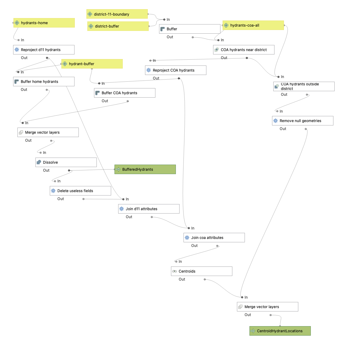
(Yellow boxes are model inputs, green are outputs, white are components of the model, which are each a simpler geospatial operation.)

Effectively what this boils down to:

1. Reproject all hydrant data to a reasonably good coordinate system applicable to Washington: NAD83 / Washington North (EPSG:2285). This is critical because buffering around a layer of points uses whatever base unit applies to the layer's CRS, and we do not want to be buffering by a hundred degrees or some such.
2. Separate out hydrants outside the possible overlap area. This was crucial because the City of Anacortes has a lot of hydrants, including many that are quite close to one another. I didn't want to accidentally merge those. (I also had to do some shenanigans to ensure that ghost hydrants didn't appear in both the in- and out-of-district subsets of the Anacortes data. Surely there's a better way to do this...right?)
3. Buffer around all hydrants by 100 feet. Based on a bit of experimentation, 100 feet felt like about the right distance – it captured most of the hydrant pairs without merging too many hydrants that were definitely separate from each other. Plus it's a nice, round, memorable number.
4. Now for the magic – I merge the two buffered datasets and dissolve any boundaries. And then I do a spatial join to get attributes from both county and city data attached to the resulting polygons. The result is some circles with just one set of attributes (where there's no other hydrant within 100 feet), and some merged circles that look sort of figure-eight-like, which will have attributes from both datasets.
5. Finally, we take the centroid of each distinct shape as the new location of the hydrants. This assumes that the two datasets are equally good approximations of the actual hydrant location, which is a bit of a guess, but hopefully a decent one.

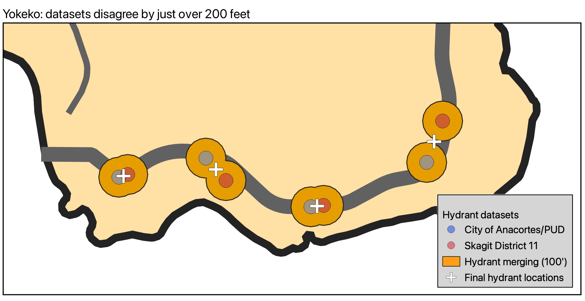
After all this, there were several edge cases that weren't quite taken care of. Things like hydrants that may or may not exist, places where I couldn't tell whether two data points were secretly the same hydrant or distinct ones, that sort of thing. I did some manual intervention on nine hydrants or hydrant pairs, some of which included actually driving around and scrutinizing blackberry bushes to see if I thought a hydrant could be hiding in there. Here are a couple sample edge cases:

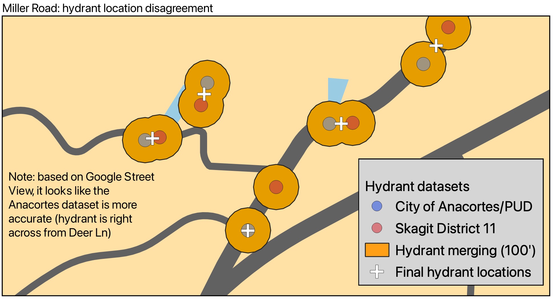
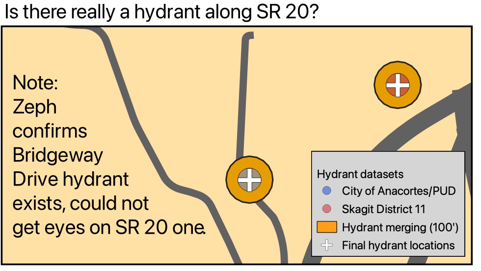
So, are there better ways to do this? Definitely! It would certainly have been faster to just manually tag hydrants as matching or not, then take centroids from there. It almost might have been faster to learn geopandas or pyqgis and just written a script to do this (I can think of several algorithmic improvements off the top of my head). But it was a fun exploration of the graphical modeler and I'm fairly happy with the result.

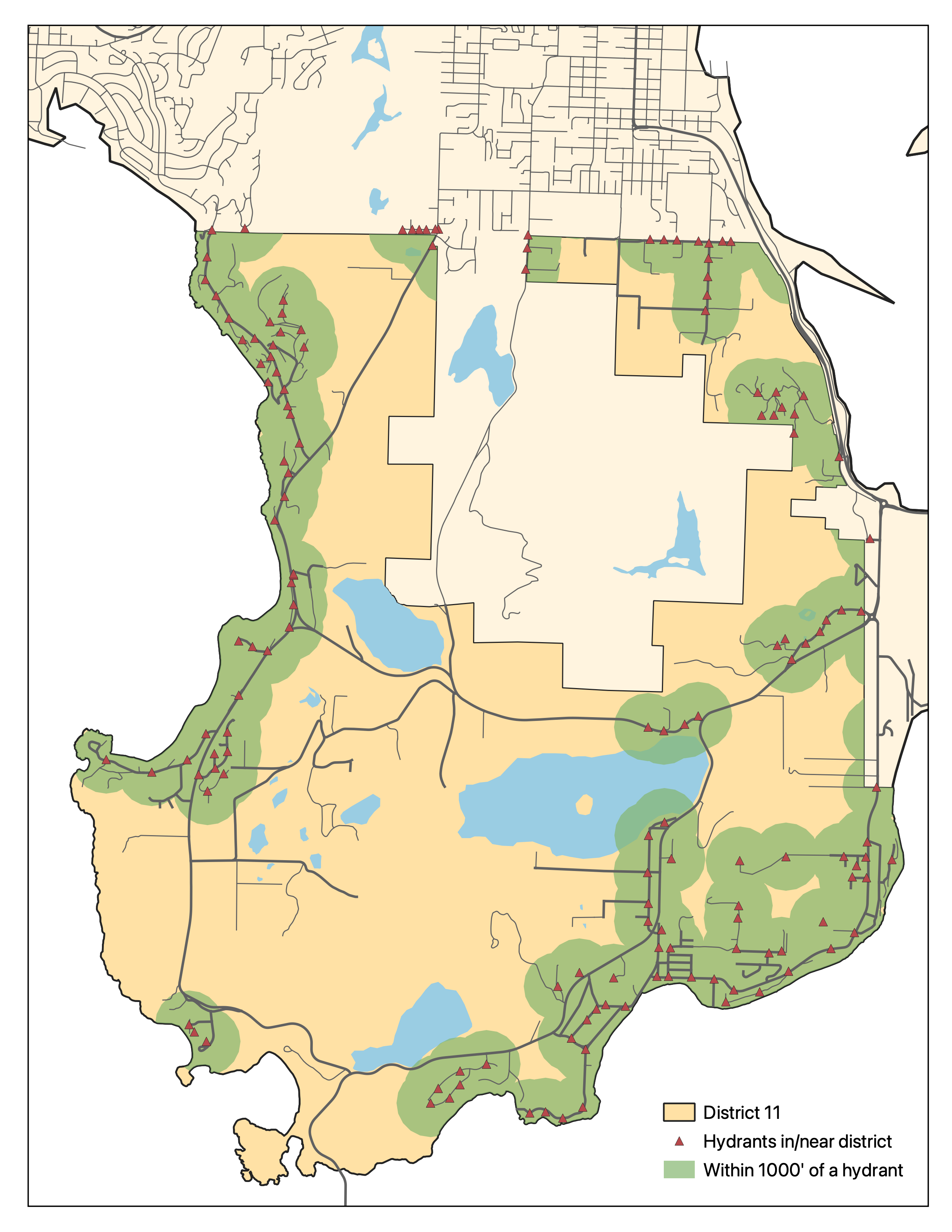
And without further ado, here's the updated district hydrants! If you want access to an interactive version of this map, shoot me an email (firstname.lastname@gmail.com) and I'll see what I can do.